Clustering technique for Redistricting
This is the final part of the Gerrymandering series in which I will discuss a clustering technique that is used to generate a district plan.
In the previous blogs, we discussed what gerrymandering is, how it is harmful for democracy and saw how gerrymandered the 2012 plan for PA was. Now, we will see if introducing machine learning into this aspect improves the plan or not. For now, we will be focussing on clustering technique.
The main goal with clustering was to create a plan in which I can get considerably compact and fair (based on voter distribution) districts while maintaining an even distribution of population across all districts. For that, I chose k-means clustering. Initially, I implemented a classic k-means clustering (i.e. just using centroids, no population criteria) to see how the results turn out.
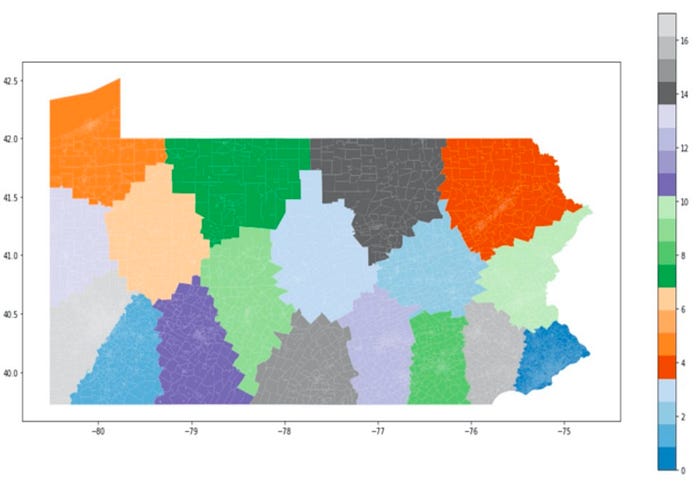
The plan seems to be pretty compact compared to the 2012 and 2018 plans. But what about population distribution?
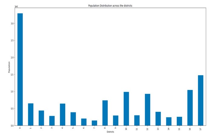
Turns out, the population distribution is bad, worse than even the 2012 plan. However, that makes sense since we did not pass any population criteria to the algorithm.
There is an interesting concept called weighted k-means, in which we use population to calculate weight. The formula is stated as

where |Cᵢ| is the population of a district and 𝛼 is used to penalize the districts with disproportionate populations. In our case, 𝛼 is between 0 and 5. Based on my analysis, the higher the 𝛼, the better the results. Once I calculate weight (wᵢ), it is used to calculate the scaling factor which then is used to calculate scaled distance. The formula is stated as the following, with 𝛽 being between 0 and 1.

Now just like classic k-means, weighted k-means also takes a few parameters such as distance, minimum population, maximum population, 𝛼 and 𝛽. In the original paper, the authors implemented Minimum pairwise distance. I tried three distance metrics, namely the great circle, Haversine, and Euclidean. The great circle did not give an impressive result. The distribution again was bad, so we rejected it. Haversine and Euclidean gave similar results. Although Heversine considers the curvature of the earth for its calculation, it did not make the result any better. Thus, I decided on the Euclidean distance metric since it was simple and was giving good results.
Other than that, it takes minimum and maximum population criteria which is used to define range for the population to vary. The range must be as small as possible. I was initially trying to use min and max population of the remedial plan (min was about 703,000 and max was about 709,000 which would have been a pretty decent range) but the algorithm was not converging. So after some hit and trial, I took minimum population as 650,000 and maximum population as 850,000. I know it’s not that great but turns it gives a pretty decent distribution (you will see it later).
Following is the plan which was generated by weighted K-means:
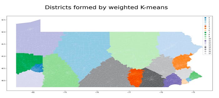
Looks pretty compact, right? But what about the population distribution?
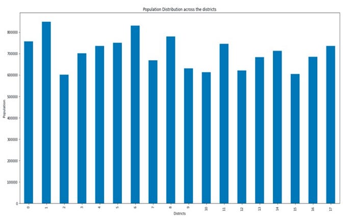
We can see the population distribution improved drastically compared to the 2012 plan. Now, let’s see how much compactness metrics improved.
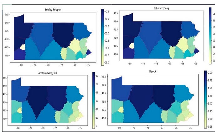
Compactness metrics have definitely improved compared to the 2012 plan. There are more darker regions in this plan compared to the existing plans but that does not give assurance as to whether the plan is good enough or not. We need to analyze fairness metrics as well.

The efficiency gap has improved, which implies that the wasted votes have been reduced. However, partisan bias and mean-median difference have not improved. There is room for improvement in those aspects.
What did I learn from this?
Using weighted K-means, we saw a great improvement in population distribution and compactness scores. Apart from that, the efficiency gap was reduced, which implies not many Democratic votes have been wasted (as I calculated fairness metrics pro-Republican). However, I couldn’t improve partisan-bias and mean-median difference, which would be my future work. What I feel is that I might need to incorporate voter distribution into the algorithm. Other than that, although there has been a great improvement in population distribution, it is still not perfect. I may need to use techniques such as a Network Flow approach to make it better.
The main motive here is to try to find a way by which we can incorporate machine learning principles into this issue and find an optimal solution. This is just a starting for that and there is room for improvement.
You can check Gerrychain in which the researchers are using Markov Chain models to generate an ensemble of states and come up with a good plan.
You can check my project here (It also contains regression analysis which helps in understanding importance of various factors which determine voter’s inclination towards a party).
References:-
- Guest, O., Kanayet, F.J. & Love, B.C. Gerrymandering and computational redistricting. J Comput Soc Sc 2, 119–131 (2019). https://doi.org/10.1007/s42001-019-00053-9
